TLDR; step size which optimizes loss after $k$ steps of minibatch SGD with batch size $B$ on realizable noiseless linear least squares problem with Hessian $H$ is the solution to the following problem.

Where $T_{\alpha,B}=(I-\frac{\alpha}{B} X^TX)$ is the mini-batch update operator with randomly sampled batch $X$, containing $B$ random observations $x$ stacked as rows. Setup borrows from Bach/Deffosez paper. Derivation assumed that $w_0$ is initialized in a way such that distribution of error=$w_0-w_\text{opt}$ is isotropic, enabling use of expectation formula (derivation, explanation)

Progress on this problem could address the problem of predicted $\alpha$ being too low for practice, possibly caused by number of optimization steps being small relative to dimensionality of the problem, making classical bounds pessimistic. We also want guidance for the batch size $B$ to use, and how to change our step size $\alpha$ when we change $B$.

Dealing with Eq $\ref{master}$ is hard, maybe can solve simpler problems?

Simplifications

• Gaussian case: if $x\sim$ Gaussian with $E[xx']=\Sigma$ and $E[x]=\mu$, can utilize the following
  $$E[xx'Axx']=\Sigma A\Sigma+\Sigma A^T \Sigma + \Sigma \text{Tr}(\Sigma A)-2\mu \mu^T \mu^T A \mu$$ ^{(recheck source around p. 435 of Seber book (pdf) or rerun Mathematica verifier)}
• optimize reduction in norm of error=$w-w^*$ instead of reduction in loss
• set $k=1$ or $k=\infty$ (focus on the first step or the last step)
• switch the order of $\text{argmin}$ and $E$

With simplifications above, we can draw random sample $X$ and solve the following problem:

Interpretation

• $\hat{\alpha}_\text{max}$: largest stable step size if we fixed $X$ and iterated steps
• $\hat{\alpha}_\text{opt}$: step size that achieves optimal single-step reduction in expected error norm for fixed $X$ under "isotropic error" assumption (ie, $k=1$)
• both step sizes are set on "per-batch" basis

Now consider expected values of these quantities as we sample random batch $X$:

I find in simulations that these these expectations harmonically interpolate between two extremes. Extremes are predicted by two "effective ranks" r and R from Srebro/Bartlett papers.

Where

and $r$ and $R$ match Definition 3 from Srebro's "Uniform Convergence" paper. (r also in occurs in many places, in Belkin's paper page 34, Nick Harvey notes, Tropp has a whole Chapter on it, Chapter 7 in survey)

These formulas give a near-perfect fit in simulations. Example with non-isotropic Gaussian in $d=200$ dimensions (code)

These two effective ranks allow us to get estimates of "critical batch size", setting of batch size $B$ such that corresponding value of $\alpha$ is halfway between two extremes.

$$B_{\text{max}}=r+1$$
$$B_{\text{opt}}=R+1$$

In simulations $B_{\text{opt}}$ seems to predict the batch size at which our batch efficiency is $\approx 0.5$ relative to SGD with batch-size 1.

Computation of batch efficiency:

• For a given batch X of size B, compute "expected reduction in error norm squared" in a single step by using $\alpha_\text{opt}$ rule to set the learning rate and isotropic error assumption (k=1), relative to what we'd expect by extrapolating from expectation of a similarly obtained reduction from a single step using batch size 1.

What we care about in practice is some heuristic to estimate the point where adding additional examples to batch doesn't help, where "doesn't help" means that 2 additional "parallel examples" (growing the batch) are worth less than 1 "serial example" (taking new SGD step with batch size 1)

We can observe in simulation some typical efficiencies observed when using these two critical batch sizes to set batch size for $X$, for various distributions and computing "batch efficiency". In the plot below, $x$ axis is dims of Gaussian, with eigenvalues $1,1/2,\ldots,1/\text{dims}$. Note that such harmonic eigenvalue decay mimics what we see in practice (Section 3.5 of NQM paper, I've observed similar in my experiments). We can see that efficiency with batch size $R+1$ is about 50%, and stays constant, while efficiency when using batch size r+1 changes with dimensions. Idea of using $r+1$ for critical batch size comes from Belkin's Fit Without Fear, page 34, but simulations show that $R+1$ is a better fit. There's a bit of a quantization error, R+1 is floating point number, so we have to round.

Average case vs bound

Solving Eq $\ref{master}$ gives a heuristic, but perhaps this approach can be used to generate bounds? Worst case becomes exponentially unlikely in high dimensions, so perhaps we can get good bounds by using  "average case+epsilon" and an assumption on the spectrum of problem. For spectrum can use

• $\lambda_i \propto \frac{1}{i^{1+\epsilon}}$, based on empirical observations on Resnet-50, Section 3.5 of NQP paper, and my MNIST experiments
• $\lambda_i \propto \frac{1}{i^{1+\epsilon}}$ from "alpha-capacity" condition
• $\lambda_i \propto \frac{1}{i \log i}$ from feature log-regularity conditions

The last two are summarized in Appendix A of Varre paper.

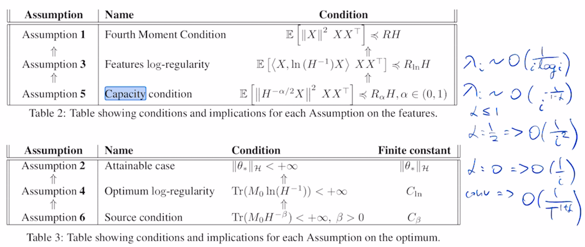
Some kind of restriction along the lines of "alpha-capacity" or "log-regularity" is required for the spectrum to be normalizable, a reasonable assumption when estimating a "finite" problem. An example of average case analysis turning into a bound is here.

Open questions

• can empirically obtained formulas be theoretically verified? Intermediate step might be to establish the following relations, for spectral/Frobenius norm of $B$ random observations $x$ stacked into batch $X$, suggested by simulations on Gaussian data. $r$ and $R$ are "effective ranks", defined in Equation $\ref{ranks}$

$$E[\|X'X\|] \le B \frac{E\|x\|^2}{r}$$
$$E[\|X'X\|_F] \approx B \frac{E\|x\|^2}{\sqrt{R}}$$

• setting above makes it possible to obtain $\alpha$ that minimizes expected error norm for extremes $B=1$ (fully stochastic step), $B=\infty$ (deterministic step), $k=1$ (best $\alpha$ for first step), $k=\infty$ (best $\alpha$ for last step). Is there a nice formula for intermediate values of B or k? Varying $B$ is possible by using Gaussian moment formulas, what about $k$? Perhaps there's asymptotic expansion for small k and for large k in the limit of dimensions $\to \infty$?
• Learning rate simulations switched order of E and argmin in Equation $\ref{master}$, is that problematic?
• Bring $H$ back into the problem – obtain $\alpha$ which focuses on population loss $\text{Tr}(T_{\alpha,B}^k H T_{\alpha,B}^k)$ instead of error  norm $\text{Tr}(T_{\alpha,B}^k T_{\alpha,B}^k)$
• Can we compute "critical batch size" when setting $\alpha$ to optimize loss instead of error? IE, set $\alpha$ to optimize loss, find $B$ for which expected reduction in population loss is about $B/2$ greater than we observe with batch size=1. Does this give significantly different results for some realistic spectra? (IE, Hessian with $1/i$ eigenvalue decay, which is what's observed in some practical problems, see Section 3.5 of Grosse NQM paper). My suspicion based on some toy simulations is that we can use either "error norm" or "loss", they would give similar results for this spectrum.
• When is analysis based on $k=1$  relevant? IE, we train a model with $d$=few billion by taking a few thousand steps, realistic case when rapid prototyping, can we bound the error we obtain by making $k=1$ assumption? (using $k=\infty$ is not relevant when number of dimensions exceeds number of steps, using "Impossibility of linear rates" section in Varre paper). The question could be – as we grow dimensionality of the problem, what is the largest number of steps $k_\text{max}$ for which the learning rate obtained from $k=1$ assumption "works"? If it grows as square root of dimension or effective rank, then maybe going with $k=1$ is OK. It it's logarithmic, then no.
• Naive estimator of $R$ is too expensive in practice because of need to estimate $\|\Sigma\|_F$. Dimensionality can be billions, so can't form outer product $xx'$. There's an efficient expectation formula using Gaussian moments. Both "naive" and "efficient" estimators overestimate $\|\Sigma\|_F$ when number of samples is small, can bias be improved?
• "efficient estimator" is not robust for non-Gaussian data, it completely fails for normalized data, what to do in such case?
• We can decide to allocate FLOP budget by either increasing batch size for fixed model size, or increasing model size while keeping batch fixed. Practitioner lore is that it's "always better" to grow model size instead of growing batch size for a fixed FLOP budget, is this true for linear least squares with fixed accuracy target? IE, BLOOM decreased loss about 100x over 12 months, so we could use "100x reduction over starting loss" as the fixed accuracy target and ask whether it's better to "increase dimensions" or "increase batch" with some assumption on spectrum of Hessian. $1/i$ spectrum is sometimes observed but not normalizable,  so perhaps use $\lambda_i=i^{-1-\eps}$

Derivations/Notation

Let our observations $(x,y),\ldots$ come from some (potentially infinite) dataset We seek $w$ such following is true for all pairs $(x,y$:
$$\langle w, x \rangle = y$$

To this effect we frame it as optimization problem with least squares objective $f(x,y)=\frac{1}{2}(x'w-y)^2$

$$w=\text{argmin}_w E f(x,y)$$

This problem has Hessian $H$, which is also the covariance of $x$: $E[x x^T]=H$.

We initialize $w_0$ randomly and apply gradient descent update to reduce gradient on randomly drawn sample $(x,y)$:

$$w_{i+1} = w_i - \alpha x (x'w_i-y)$$

Let $w^*$ indicate the solution to this problem and let $e_i$ be the error at step $i$

$$e_i = w_i - w^*$$

We have the following:

$$e_{i+1}=(I-\alpha xx')e_i = T_\alpha e_i$$

Let $H=E[xx']$, $C=E[\|e_0\|^2]$, we have the following for our starting $L_0$

$$L_0 = E_{w_0} [e_0^T H e_0] = C\cdot \text{Tr}H$$

We are able to apply $\text{Tr}$ result by assuming that distribution of $w_0-w^*$ is isotropic which encodes our initial ignorance of location of the optimum. For derivation see this post

Now we get the following expected loss after $k$ steps of gradient descent

$$L_k = E_{w_0} [e_0^T T_\alpha^k H T_\alpha^k e_0] = C\cdot \text{Tr} (T_\alpha^k H T_\alpha^k)$$

Real life problems are typically normalized (ie, when training language models, $1<L_0<100$ regardless of model/dimension), hence we only care about relative reduction in loss. Hence find $\alpha$ that minimizes the following quantity:

$$L_k = \text{Tr}(T_\alpha^k H T_\alpha^k)$$

Too hard, so find $\alpha$ which maximizes the following simpler objective instead:

$$\|e_k\|^2 = \text{Tr}(T_\alpha^k T_\alpha^k)$$

Our operator $T_\alpha=(I-\alpha xx^T)$ takes a gradient step for 1 observation. In practice we typically take several gradient at once. To model this, we can stack multiple samples $x$ into data matrix $X$ with $B$ examples as $B$ rows. Our gradient update operator takes the following form:

$$T_{\alpha,B}=\left(I-\frac{\alpha}{B} X^T X\right)$$

Division by $B$ follows the convention in machine learning which divides by the number of examples. This explains the "linear learning rate scaling" rule – for small $B$, doubling $B$ means we need to double $\alpha$. At some point this rule breaks down – this is connected to the "critical batch size" phenomenon.

Now, the optimal step size which minimizes loss after $k$ steps is the solution of the following problem:

while optimal step size which minimizes error norm after $k$ steps is the solution of the following problem: