Gradient descent under harmonic eigenvalue decay

Consider using gradient descent to minimize a quadratic objective with Hessian $H$.
$$\begin{equation} f(w)=\frac{1}{2}(w-w_*)^TH(w-w_*) \label{loss} \end{equation}$$We can specialize by letting $H$ have $i$'th eigenvalue proportional to $\frac{1}{i}$ . This decay was observed in some convolutional network problems and conjectured to hold more generally, see Section 3.5 of Noisy Quadratic Model paper.
Because relative loss trajectory of a randomly initialized gradient descent is invariant to rotation and scale of our quadratic objective, we can assume $H$ is diagonal with norm 1 without loss of generality, giving following simple closed form for loss after $t$ steps. Assuming $w_*=0$, we get result below.
$$\begin{equation} L(t)=\sum_{i=1}^n (1-\alpha h_i)^{2t} h_i w_0^2 \label{loss2} \end{equation} $$For derivation, see Gradient Descent on a Quadratic post
Each starting point $w_0$ gives a different loss trajectory, but you can show that in high dimensions and diagonal Hessian, almost all loss trajectories cluster around the trajectory for starting point $1,1,1,\ldots,1$.

This means that it's sufficient to analyze behavior of the following equation:
$$f(s,n)=\frac{1}{H_n}\sum_{i=1}^n \left(1-\frac{1}{i}\right)^{2s}\frac{1}{i}$$
This $H_n$ term refers to $n$th Harmonic number, and is there to make sure initial loss is constant regardless of dimensionality, which is the case for real-life models.
This equation can be better understood using asymptotic expansions which were provided to me by George Nemes on math.SE. We can summarize it as follows:
1) Loss initially drops sharply as negative log
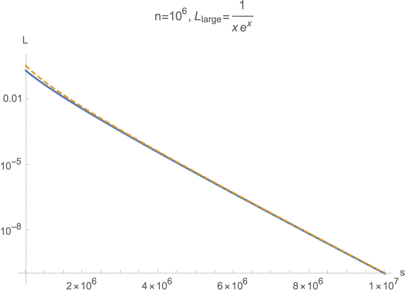
2) Followed by slightly-super-exponential rate $1/(x e^x)$.
3) Eventually switching into traditional "exponential" decay.
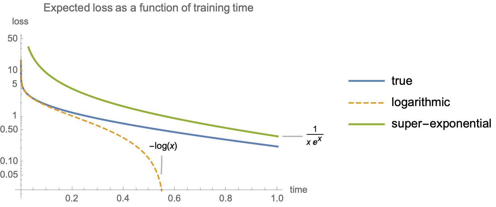
x-axis in this graph gives steps normalized by the number of dimensions. This means that as dimensionality grows, more training steps exhibit the ultra-rapid logarithmic loss decay.
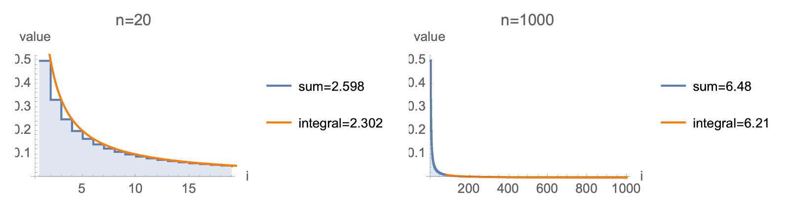
The trick to obtain this is to replace our summation with an integral:
$$\begin{equation}L(s)\approx \int_{i=1}^n \left(1-\frac{1}{i}\right)^{2s} \frac{1}{i} \mathrm{d}i\label{defInt}\end{equation}$$
Integral approximation corresponds to taking the area under smooth curve whereas the sum adds up area under step function below. Curve flattens out for large $n$, so integral approximation becomes more accurate as $n$ increases.
For most values, $1/i$ is small, hence we can approximate $1-1/i$ as $\text{exp}(-1/i)$, obtained from series expansion of $\text{exp}(-x)$
$$\text{exp}(-x)=1-x + O(x^2) $$
Use this approximation to simplify the integral in Eq $\ref{defInt}$
$$L(s)\approx \int_{1}^n \frac{\text{exp}(-2s/i)}{i} \mathrm{d}i\approx E_1\left(\frac{2s}{n}\right)$$
Here $E_1$ is the exponential integral. This approximation is valid when the number of steps $s$ grows slower than dimensionality squared $n^2$, confirmed by George Nemes here.
We can plot integral approximation of loss against exact loss after s steps and see that this approximation tracks true loss closely.

Now we can compute series expansion of $E_1$ at 0 and at $\infty$ to get small $s$ and large $s$ approximations. Furthermore, you can obtain the number of steps needed to reach target for these two regimes by applying asymptotic inversion to exponential integral, as documented here.
Define $x$ as the argument of $E_1$ in the last equation to get the expression of loss in terms of exponential integral.
You can think of $x$, the value inside exponential integral, as the "dual epoch" – steps normalized by number of parameters rather than by number of examples for regular epochs.
As you see in worst case analysis (post), you will need to run for O(n) steps for worst case scenario starts to depend on the smallest eigenvalue. Meanwhile, it will take more than $n^2$ steps for the typical case to become sensitive to the smallest eigenvalue.
Expanding $E_1(x)$ at $0$ and at $\infty$, we get the following small-x and large-x approximations.
$$L_\text{small}(x)\approx -\log(x)$$
$$L_\text{large}(x)\approx \frac{1}{x e^{x}}$$
Initial decay is logarithmic and this approximation is valid perhaps for the first $n/20$ steps.

Meanwhile, large-s approximation becomes good as the number of steps approaches the number of dimensions.
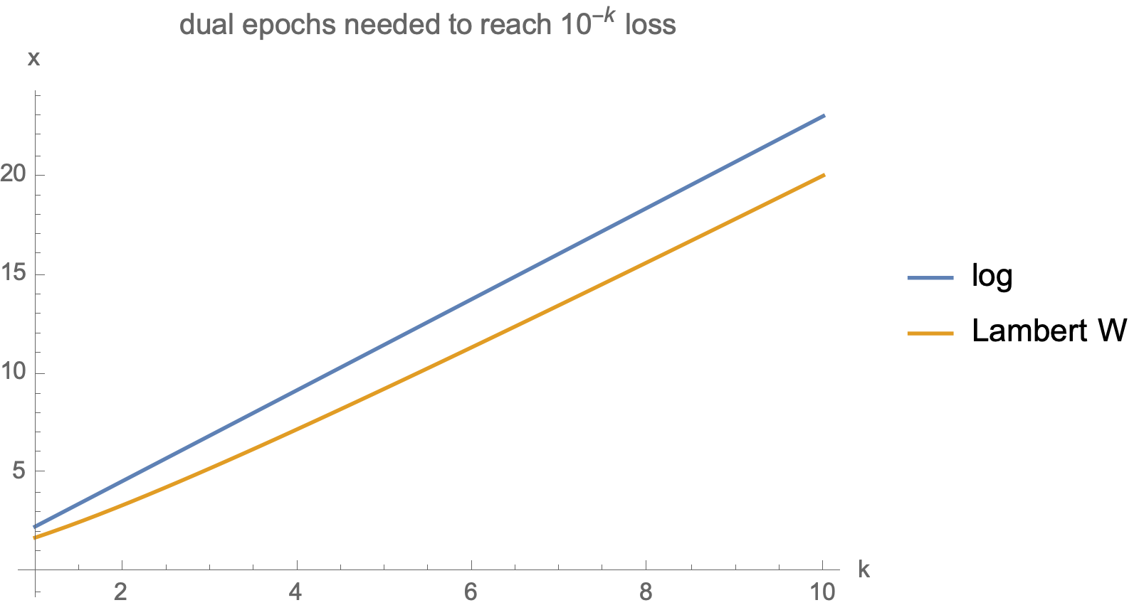
The function that solves for the number of steps needed to reach a given loss is known as Lambert W function, or the "product log" function. We can use log as an upper bound.
For instance consider solving for the steps needed to achieve $10^{-k}$ loss: