Gradient descent under harmonic eigenvalue decay: worst-case analysis

Consider minimizing the following objective using gradient descent with learning rate $\alpha$ and $x\in \mathbb{R}^n$
$$\begin{equation}y=x^T H x \label{loss} \end{equation} $$Where $H$ is Hessian matrix with $i$'th eigenvalue proportional to $\frac{1}{i}$ . This decay was observed in some convolutional network problems and conjectured to hold more generally, see Section 3.5 of Noisy Quadratic Model paper.
Because gradient descent is rotationally invariant, we can take $H$ to be diagonal with norm 1. Harmonic eigenvalue decay then corresponds to the following matrix.
$$H=\left(\begin{array}{ccccc} 1& 0 & 0 & \ldots & 0\\ 0 & \frac{1}{2} & 0 & \ldots& 0\\ 0 & 0 & \frac{1}{3} & \ldots & 0\\ \ldots & \ldots & \ldots & \ldots & \ldots\\ 0 &0 &0 &\ldots & \frac{1}{n} \end{array} \right)$$Below we show that worst-case loss after $s$ steps for large $n$ is proportional to $1/s$
$$ \begin{equation} y_\text{worst}^s\approx \frac{1}{s} \end{equation} $$Take starting point to lie on the unit circle and consider the loss after $s$ steps
You can show that worst-case scenario after $s$ steps picks a starting point where just one of the coordinates is non-zero, this coordinate depends on $s$. Below we can see in 2D how the worst case starting point changes depending on how many steps we take.

Initially we get worst-case loss by starting with $(1,0)$, but eventually switch to $(0,1)$ which is the direction of smallest eigenvalue. Also, note that as we keep iterating, direction of gradient step aligns with the direction of smallest eigenvalue, so this rate determines eventual rate regardless of starting position.
Hence, eventually, our gradient descent is plodding along the smallest eigenvalue direction $e_n$, shrinks the distance by factor of $1-\lambda_n$ at each step. What if we used higher learning rate instead of $1$?
Unfortunately, if we use learning rate higher than $2/\lambda_1$, gradient descent becomes unstable and diverges along the direction of the largest eigenvalue $\lambda_1$.
Hence, asymptotic convergence rate is determined by the ratio of the largest and smallest eigenvalues, known as the condition number.
This is the classical analysis, but it often doesn't apply to practical high dimensional problems because reaching asymptotic regime requires unrealistic number of steps in high dimensions.
Consider again worst case direction after $s$ steps of gradient descent in 2 dimensions.
Now consider the same graph in 50 dimensions, visualizing worst case minimization path, along with some paths starting with random positions.
Solving for the direction producing worst-case loss after $s$ steps we get a vector with all 0s and a single 1 at the following position
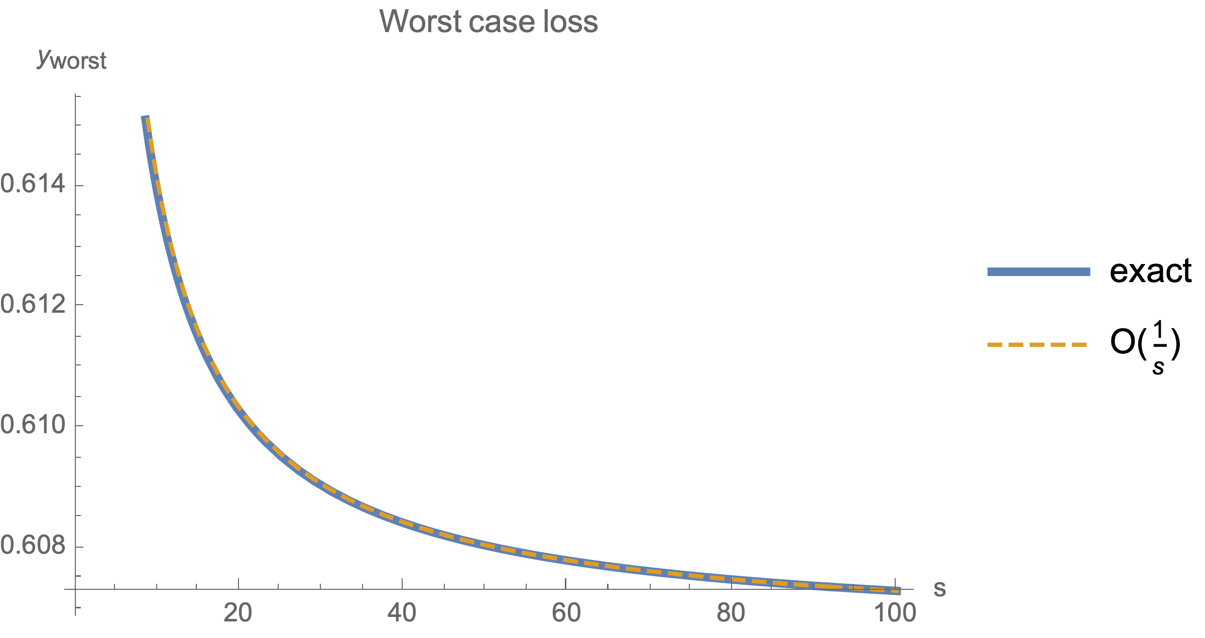
$$ \begin{equation} i = \begin{cases} 2s+1 & s<\frac{n}{2} \\ n & \text{otherwise } \end{cases} \end{equation} $$ $$ x_\text{worst}=\langle 0, 0, \ldots, \underbrace{1}_{\text{i}}, \ldots, 0\rangle $$Now for this starting position, compute gradient descent estimate after $s$ steps, substituting this into equation of loss, Eq $\ref{loss}$, and take 1st order Taylor approximation, we get
$$y^s_\text{worst}\approx \frac{8 s+1}{8 \sqrt{e} s} = O\left(\frac{1}{s}\right)$$
Note that when dimensionality $n$ exceeds number of 2*steps, worst case analysis does not depend on $n$