Value of quadratic form on a unit circle

Suppose we sample $(x_1,x_2)$ uniformly from unit circle, are interested in the distribution of the following quantity.
$$ X=\left(\begin{array}{cc}x_1& x_2\end{array}\right)\cdot \left(\begin{array}{cc} 3&0\\ 0&1\\ \end{array}\right)\cdot \left( \begin{array}{c}x_1\\x_2\end{array} \right) $$This is the value of a quadratic form evaluated at a random point on the unit circle.
What distribution does it follow? We can write this random variable as a linear combination of eigenvalues and a new random variable $y=(x_1^2,x_2^2)$
$$X=\lambda_1 x_1^2 + \lambda_2 x_2^2$$ $$X=\lambda_1 y_1 + \lambda_2 y_2$$Now our target variable is a linear combination of components of random variable $y$. What distribution does $y$ follow? Notice that if the original points lie on a circle, their squares add up to 1, hence squared coordinates lie on the simplex.
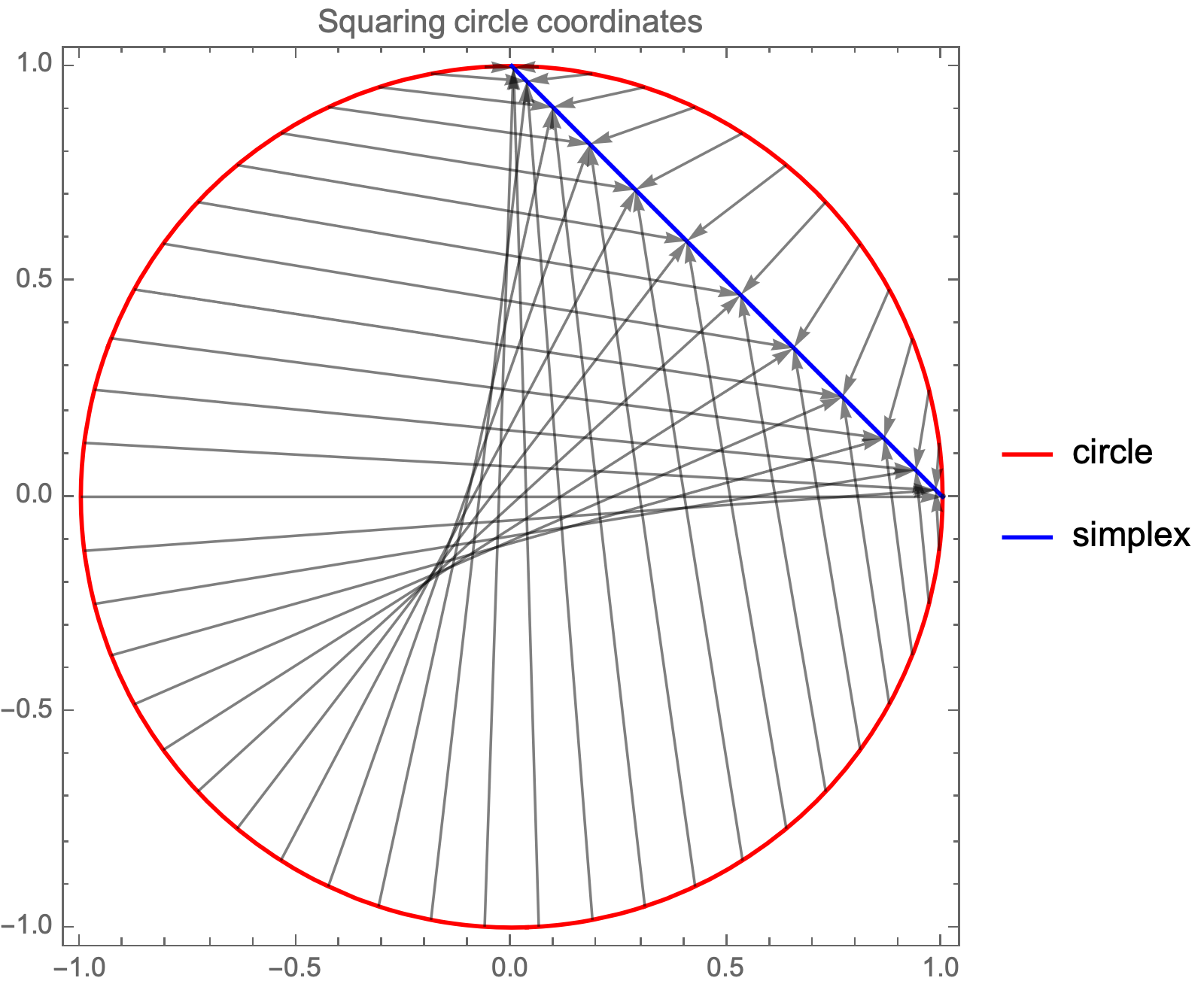
You can see that points towards the edges of the simplex are spaced more closely together corresponding to higher density. You can see this effect if we look at 3d histogram of original and transformed distributions.
Similarly, squaring coordinates of points distributed on the surface of a sphere maps the points to the 2-dimensional simplex, giving distribution peaked at the corners.
These contours may look familiar as the contours of the Dirichlet distribution. You can show this rigorously by using change of coordinates equation. Recall that when applying change of coordinates function $f$ to constant density, new density is proportional to the determinant of the inverse Jacobian of $f$.
$$\begin{equation} \begin{split} x \Rightarrow &f(x)\\\\ \mathrm{d}G(x) \Rightarrow &|df^{-1}(x)| \end{split} \end{equation} $$Here's our transformation and the inverse
$$\left( \begin{array}{ccc} x_1 \\ x_2 \\ \ldots\\ \end{array} \right) \xrightarrow{\mathit{f}} \left(\begin{array}{ccc} x_1^2 \\ x_2^2 \\ \ldots \end{array} \right) $$ $$ \left( \begin{array}{ccc} y_1 \\ y_2 \\ \ldots\\ \end{array} \right) \xrightarrow{\mathit{f^{-1}}} \left(\begin{array}{ccc} \sqrt{y_1} \\ \sqrt{y_2} \\ \ldots \end{array} \right) $$Now we can write the Jacobian and its determinant
$$ df^{-1}\propto \left(\begin{array}{ccc} \frac{1}{\sqrt{y_1}} & 0 & \ldots\\ 0 & \frac{1}{\sqrt{y_2}} & \ldots\\ \ldots & \ldots & \ldots \end{array} \right) $$ $$ |df^{-1}|\propto \frac{1}{\sqrt{y_1}} \frac{1}{\sqrt{y_2}} \cdots $$This PDF corresponds to Dirichlet(1/2,1/2). Therefore our quadratic value is distributed as a weighted linear combination of Dirichlet random variable, eigenvalues of the quadratic forming the weights of the linear combination.
This distribution was studied in Provost, Serge B., and Young-Ho Cheong. 2000. “On the Distribution of Linear Combinations of the Components of a Dirichlet Random Vector.” (link).
There's no nice closed form for this distribution, plotted below for weights from our example problem.
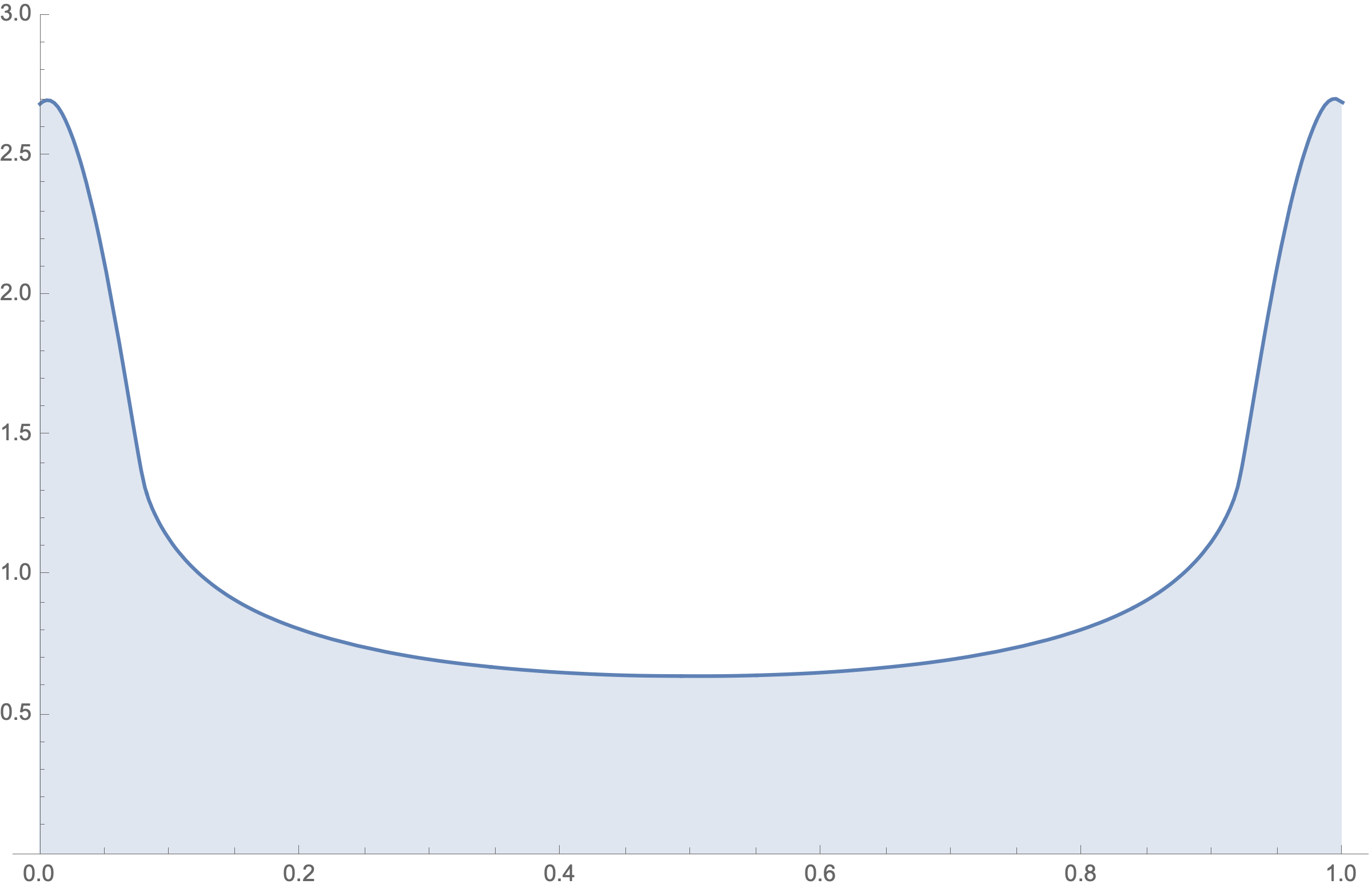
However, there's a nice expression for the first two moments, derived here
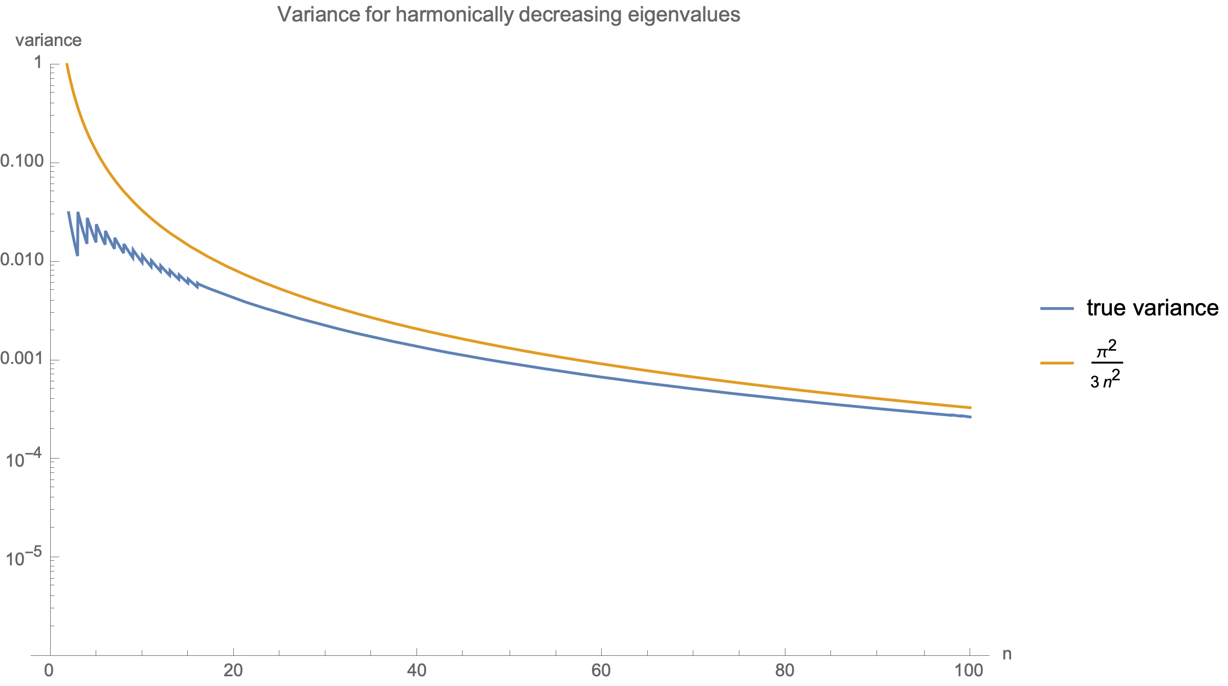
$$E[X]=\frac{1}{n}\sum_i \lambda_i$$ $$\text{var}[X]=\frac{1}{n^2(n+2)}\sum_{i,j}(\lambda_i-\lambda_j)^2$$It is instructive to consider how this behaves for $\lambda_i=\frac{1}{i}$.
$$\begin{equation} \begin{split} E[X]= O\left(\frac{\log n}{n}\right)\\\\ \text{var}[X] = O\left(\frac{1}{n^2}\right) \end{split} \end{equation} $$A non-asymptotic upper bound for variance is $\frac{\pi^2}{3n^2}$ derived here.
Related calculation shows the variance of gradient descent estimate after $s$ steps here.