• Left preconditioning refactors examples to be uncorrelated and on the same scale. Examples: Affine Projection algorithm, normalized LMS, Kaczmarz, normalized SGD.
• Right preconditioning refactors features to be uncorrelated and on the same scale. Examples: Recursive Least Squares, Newton Method, feature normalization.
• Most popular ML optimizers can be viewed as a form of right preconditioning, with preconditioner derived from gradient covariance. Classical preconditioners instead rely on Jacobian covariance. Unlike gradient covariance, Jacobian covariance does not decay to zero at convergence, ensuring a consistent learning rate over time.

Suppose you want to solve the following $m\times n$ matrix equation

You can think of it as a system of $m$ equations where coefficients of each equation are arranged as rows $a_i^T$.

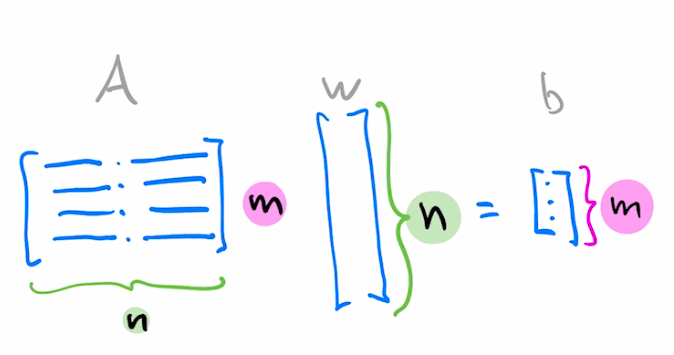
To solve this system using an iterative method, pick some loss function $f_i$ providing a scalar measure of the discrepancy between two sides of $i'th$ equation. Our $m\times n$ linear problem $Aw=b$ hence reduces to a minimization problem in $n$ dimensions with $m$ examples. To solve, minimize the following:

$$\sum_i^m f_i(a_i^T w )$$

Choose $f_i(y)=\frac{1}{2} (y-y_i)^2$ and perform one gradient descent step per element of this sum. This is the SGD algorithm, also known as the LMS filter in Signal Processing literature.

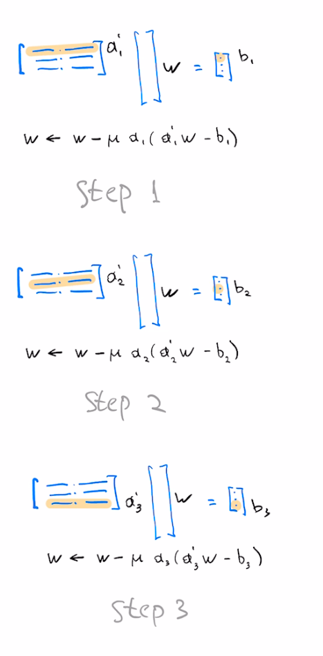
We may alternatively perform a full gradient update by considering all entries of the loss at once, aka "full-batch gradient descent". This gives us the following update:

$$w = w - \mu A^T(Aw-b)$$

In Linear Solver literature this is known as the Richardson iteration.

Gradient descent and SGD perform best on a problem which is "perfectly conditioned", corresponding to all features/examples being uncorrelated and on the same scale. Fast convergence of a cheap iterative method makes it an "easy" problem. Goal of preconditioning is to linearly transform our problem to make it "easy".

Left preconditioning

Consider multiplying both sides of the equation by $L$ on the left, aka Left Preconditioning.

Solution of this system is the same as the solution of the original system, but it can be easier for gradient descent to optimize. Suppose we take $L=A^{-1}$. In this case our iterative procedure converges right away, while $L=I$ produces the original slow Richardson iteration. These two choices can be seen as the extremes of the trade-off between "Algebraic" and "Iterative" methods.

• Algebraic methods:  time depends on dimensions of $A$ but does not depend on entries of $A$.
• Iterative methods: time depends on entries of $A$, but could be independent of dimensions of $A$ (ie, for sparse $A$)

For general choice of $L$, our SGD update equation is the following

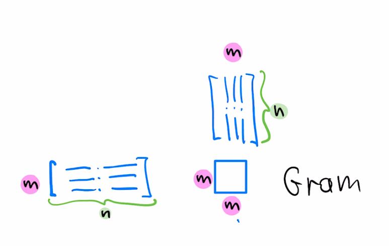
For the case of symmetric $A$, the choice of left preconditioner $L=A^{-1}$ corresponds to augmenting our SGD update with $L^T L=(AA^T)^{-1}$, ie, inverse of the Gram matrix

For the case of our dataset being large, we may consider only using $k$ rows of $A$ to form the preconditioner

Using k rows seen so far at k'th step of optimization gives the Affine Projection algorithm. Using $k=1$ (only the current row) corresponds to normalized LMS, also known as the Kaczmarz algorithm. Equivalently, $k=1$ corresponds to diagonal left preconditioner with reciprocals of norms of $a_i$ on the diagonal.

This preconditioner modifies gradient update with each gradient normalized by the squared norm of the corresponding example.

$$w = w - \mu  \frac{1}{\|a\|^2} a (a^T w-b)$$

Right preconditioning

To apply the right preconditioner, we define $u=R^{-1}w$ and solve the equivalent equation for $u$

$$ARu=b$$

Gradient descent is not invariant to linear transformations, and gradient descent in the space of $u$ corresponds to the following update in the original space:

If we set $RR^T=(A^T A)^{-1}$ this method corresponds to Newton update step since $A^T A$ is the Hessian of our optimization objective.

Because of extra degrees of freedom, there's more than one $R$ which corresponds to Newton step, known as "whitening transformation". Said another way, $R$ is an $n\times n$ matrix which transforms the space to remove correlations among $n$ features and makes sure these features have the same scale.

A diagonal approximation to the whitening preconditioner would have reciprocals of "column norms" as diagonal entries, which corresponds to normalizing coordinates to have the same scale.

Note that for each $A$ there's a corresponding "transposed" or "dual" problem:

$$A^T w = b$$

Left preconditioner which makes original problem "easy" is identical to the right preconditioner which makes the dual problem easy. This should make sense – left preconditioner normalizes examples, right preconditioner normalizes features. Transposing $A$ switches the role of examples and features.

Similarly, SGD on the original problem is equivalent to coordinate descent on the dual problem, hence techniques that improve coordinate descent will also improve SGD.

Another connection between original problem and its dual is that corresponding optimization problems have the same spectra (ignoring irrelevant zero eigenvalues in the larger matrix). Consider Hessians of original problem $H$ and the dual problem $H_d$

$$\begin{align}H&=&A^T A\\H_d&=&A A^T\end{align}$$

This follows from the fact that $AB$ and $BA$ have the same spectrum and can be shown algebraically. This commutativity property implies that preconditioning on the left or on the right has equal capacity to improve the condition of the corresponding optimization problem.

If we let $w_*$ indicate the position of optimal $w$ and $\hat{b}=A w$ the vector of current predictions, then we can consider the following two quantities as dual to each other.

The first gives discrepancy in the "weight" space, the second gives discrepancy in the output space. The latter is also known as the residual. One step of gradient descent in realizable (aka interpolation) regime updates each of these quantities in a surprisingly simple fashion

These recursions are good starting points to analyze convergence of SGD, first is Eq 2.1 in "Averaged Least-Mean-Squares" paper and second is Eq 2.2 in "Low-rank structure" paper

Recall that Newton method corresponds to right-preconditioned gradient descent with preconditioner R such that

$$RR^T=(A^T A)^{-1}$$

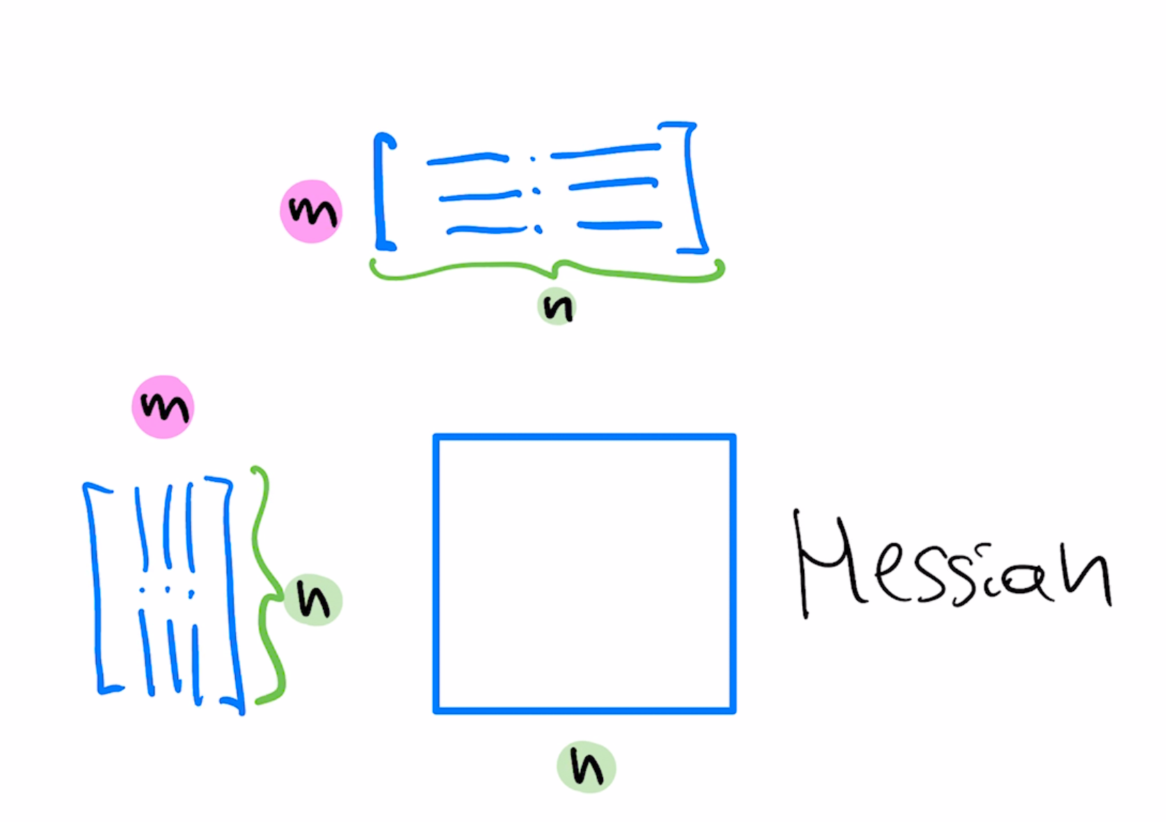
For connection to whitening, note that since examples $a$ are arranged as rows of $A$, $A^T A$ is proportional to the covariance matrix of $a$. Note that even though $A^T A$ is often called the covariance matrix, it is technically the "second-moment" matrix.  

Finding $R$ which recovers Newton method preconditioner is equivalent to finding a linear transformation which whitens $a$, ie, find transformation $R$ which makes transformed random vector have identity covariance:

Several choices of $R$ produce such whitening. You can obtain $R$ directly from eigendecomposition of $A^T A$, corresponding to PCA whitening. Alternatively, you can utilize definition of whitening as the transformation which "decorrelates" coordinates.

More specifically, do one of the following:

1. Fit a linear predictor of $k$th coordinate of $a$ based on $k-1$ coordinates using least squares. Coefficients form $k$th column of R, aka Cholesky whitening.
2. Fit a linear predictor of $k$th coordinate based on all other coordinates using least squares. See notebook, colab and Section 5.6 of "High-Dimensional Covariance Estimation" by Pourahmadi.

Because of duality, similar whitening view applies to left preconditioning. Just as right preconditioner aims to come up with new coordinate system that decorrelates coordinates, left preconditioning comes up with a view of the dataset which decorrelates examples.

Using whitening view of preconditioning, we can write the Newton step as follows

Here, i'th row of matrix $B$ contains coefficients needed to predict $i$th component of $A$ from remaining components and $D_2$ is a diagonal matrix containing total residuals squared of corresponding components left over after subtracting the predicted value.

This means that applying Newton update can be done as follows:

1. For each coordinate of each example x, subtract the predicted value by using all other coordinates of this example, using linear predictor fit with least squares to all data, producing new data matrix: $A_2'=(I-B)A'$
2. This kind of normalization will make different features have differing magnitudes, so you normalize each feature by feature norm squared. $A_3'==D_2^{-1} A_2'$. This is analogous to Kaczmarz/normalized LMS but applied to features rather than examples.
3. Finally apply regular Richardson iteration using this transformed data for the main term (but not the residual term): $w=w-A_3' (Aw-b)$

Note that $(X'X)^{-1}X'$ is also known as the right-pseudoinverse of $X$

There's also a one-sided version, which is more convenient in case you need square roots. See this discussion on stats.SE

We can map concepts of least-squares preconditioning to general optimization.

Consider gradient $\nabla J$ of a general objective $J=f(g(w))$ with predictor $g$ and loss $f$

$$\begin{align}
J&=&f(g(w))\\
J'&=&f'g'\\
\nabla J&=&(J')^T=\nabla g \nabla f
\end{align}$$

In our original least squares formulation, f is the least squares loss, and g is the linear predictor. We can identify these parts in the formula of the LMS update

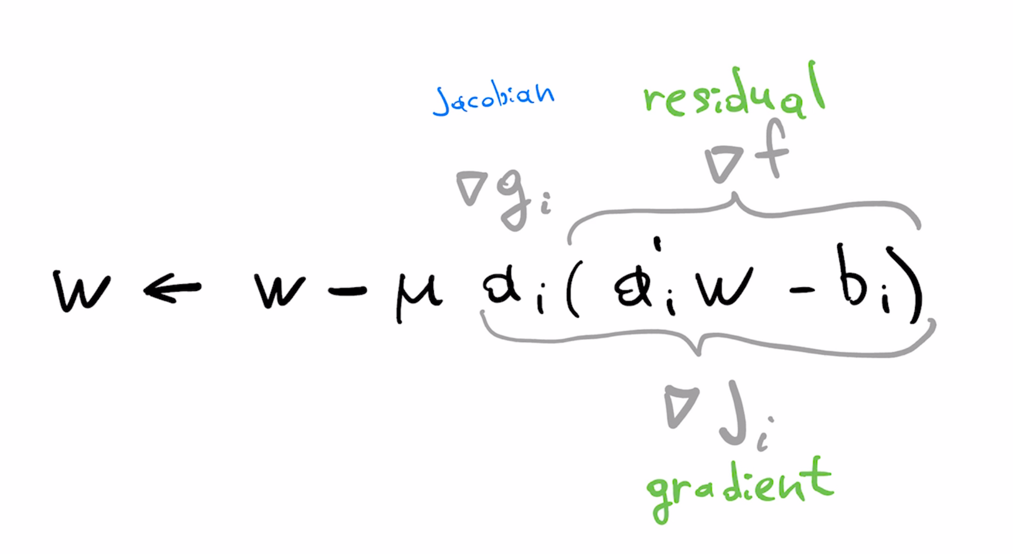
With some abuse of terminology, we can view the gradient as the product of the Jacobian and the residual. Gradient of the loss $\nabla f$ is the "residual" while gradient of predictor $\nabla g$ is the (per-example) Jacobian, matching terminology used here.

With this we can see that to get the $A$ matrix from least squares we would stack our Jacobians as rows

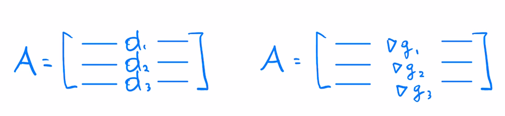
Per-example gradients matrix $B$ in least-squares case is similar to $A$, except each row is weighted by scalar residual, indicating how far off the prediction is from the target value.

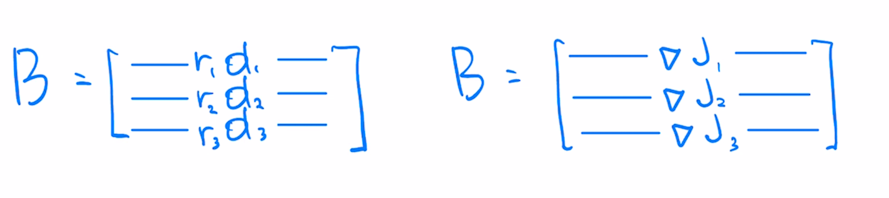
Machine learning preconditioners can be viewed as right preconditioners constructed from the covariance of gradients $B^TB$. Classical preconditioners like Newton's use covariance of Jacobians $A^TA$

Contrast the effect of using gradients matrix $B$ in place of Jacobians matrix $A$ for right-preconditioned gradient descent

You can see that the first update has a problem in realizable case because gradients $\nabla J$ converge to 0. Take scalar case. As gradient $\nabla J$ approaches 0, step length is $1/\nabla J$ so it approaches infinity. To avoid this you could take square root, which keeps step length finite in the limit

Approximating this preconditioner with a diagonal matrix produces Adam and RMSProp algorithm. More involved block approximation gives the Shampoo algorithm. Note that taking of square root doesn't fully solve the convergence issue, there are examples where Adam provably diverges.

Multi-class formulation

To convert multi-class predictors to least-squares formulation we would treat each class predictor as a separate regression problem, and stack corresponding per-example/per-class Jacobians as rows.

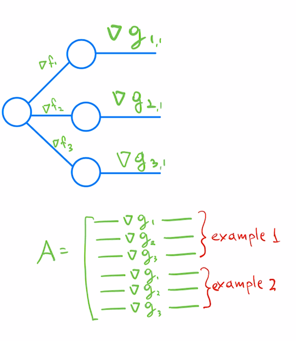
In a reverse autodiff system like PyTorch, you would get the second row of this matrix by using the following pseudo-code

y=predictor(example1)
y.backward([0,1,0,...])
predictor[0].W.grad.flatten()

To make this efficient, you could batch backward calls like this, reducing k examples x o classes to a single backward pass. Then use standard tricks for "per-example gradients" to get corresponding rows.

If your preconditioner is derived from covariance like $A^T A$, you don't need all the rows for a good approximation. In particular, you get an unbiased estimate by adding up subsets of rows with random +1/-1 weights and computing covariance from this smaller matrix.

This means you can do a single backwards call per example with something like y.backward([1,-1,1,...]). You can batch this to have similar complexity to regular gradient computation. This is the trick used by implementations of KFAC or Gauss-Newton methods.

Not aware of any existing implementations, but the following would be obvious things to try:

• Instead of normalizing coordinates by square root of "variance" of example-wise gradients, normalize coordinates by "variance" (second moment) of example-wise Jacobians. This would give the classical diagonal right preconditioner.
• Instead of normalizing gradients by their norm, normalize per-example gradients by the norm squared of the Jacobian part. This would correspond to the classical diagonal left preconditioner
• For a batch of k example-wise Jacobians, decorrelate them by dividing them on the left by $k\times k$  Jacobian Gram matrix. Multiply decorrelated rows by original residuals and add together to get updated step direction. This gives a block left preconditioner, analogous to Affine Projection algorithm.