Gradient descent on a quadratic

Consider minimizing a simple quadratic using gradient descent, assuming it attains 0 at optimum $w_*$
$$\begin{equation} f(w)=\frac{1}{2}(w-w_*)^TH(w-w_*) \label{loss0} \end{equation}$$This kind of problem is sometimes called linear estimation problem because we are trying to solve for the point where $\nabla f(w)=0$, and the gradient is linear function of parameters
$$\nabla f(w)=H(w-w_*)$$
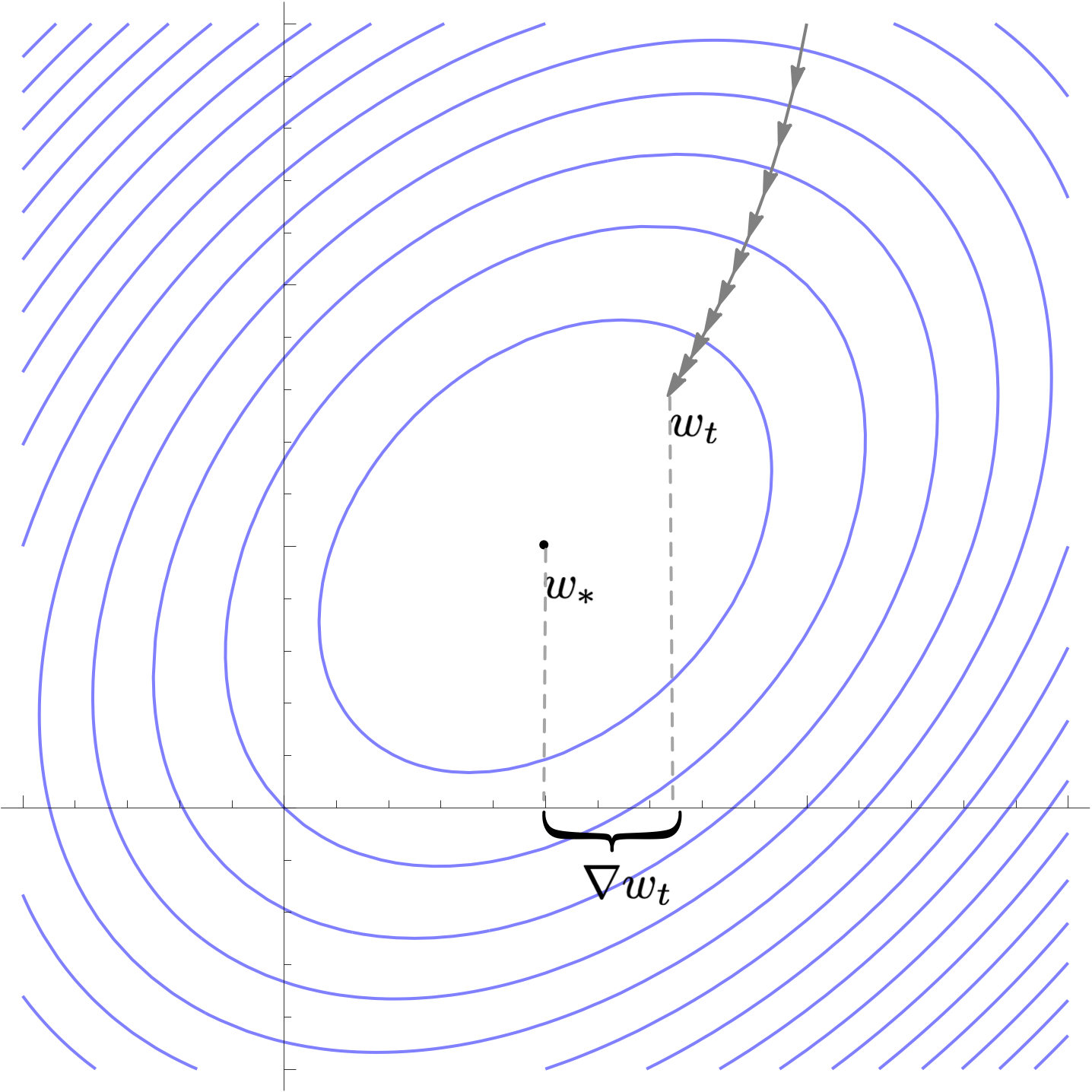
Define the difference between current parameter and optimal parameter
$$\nabla w_{t} = w_t - w_*$$
A single step of gradient descent with learning rate $\alpha$ updates this quantity as follows
$$\nabla w_{t+1} = (I-\alpha H)\nabla w_t $$
Note that gradient descent is invariant to translations, so we could assume $w_*=0$ for notational simplicity.
In which case we get $\nabla w_t = w_t$ and our weight vector at step $t$ is the following
$$w_t = (I-\alpha H)^t w_o$$
Gradient descent is additionally invariant to rotations, so we can assume that Hessian is diagonal without loss of generality. GD with momentum is also invariant, but diagonally preconditioned methods like RMSprop and Adam are not.
Here's a visualization of the path of Gradient Descent and RMSProp on quadratic minimization problem after applying rotation of coordinates
Because of this rotational invariance we can assume that Hessian is diagonal, so $i$th coordinate of the weight vector at step $t$ can be written as follows
$$\begin{equation} w^t_i = (1-h_i)^t w^0_i \label{wi} \end{equation}$$When the Hessian is not diagonal, the formula still holds, but $h_i$ refers to $i$th eigenvalue of the Hessian rather than $i$th diagonal value.
Additionally, if we only care about relative decrease in loss rather than absolute values, gradient descent is invariant to scaling of the objective. Below is visualization of gradient descent path after multiplying objective and learning rate by some constant. Absolute values of loss changes, but the relative decrease in loss does not.
Similar invariance holds if we scale starting point by a constant factor.
This means that when analyzing quadratic gradient descent, we could restrict attention to Hessians with a convenient norm, and also assume that starting position is normalized
Now lets obtain a simplified expression for loss after $t$ steps. Plugging estimate after $t$ steps $\ref{wi}$ into expression of loss $\ref{loss0}$ we get the following expression for loss after $t$ steps
$$\begin{equation} L(t)=\sum_{i=1}^n (1-\alpha h_i)^{2t} h_i w_0^2 \label{loss2} \end{equation} $$When our starting position lies on a circle with radius $\sqrt{n}$, we can show that average loss after $t$ steps is given by the following (see Value of quadratic form note)
$$\begin{equation} L(t)=\sum_{i=1}^n (1-\alpha h_i)^{2t} h_i \label{loss3} \end{equation} $$This is equivalently the loss of gradient descent with a starting point $w_0=\langle 1, 1, 1, \ldots, 1\rangle$ which is special because it becomes increasingly representative of typical gradient descent trajectories as $n$ increases.
We can further simplify this expression by noting that in typical optimization problems, Hessian eigenvalues decay, so $1-\alpha h_i$ is small for most $i$. This allows us to substitute approximation $1-x \approx \exp(-x)$
$$\begin{equation} L(t)\approx\sum_{i=1}^n \exp(-2\alpha t h_i) h_i \label{loss4} \end{equation}$$In high dimensions, the sum above could be approximated with an integral
$$\begin{equation} L(t)\approx\int_{1}^\infty h(i) \exp(-2\alpha t h(i)) \mathbb{d}i \label{loss5} \end{equation}$$If we normalize Hessian to have trace norm 1 and start at $w_0=(1,1,\ldots)$, then eigenvalues add up to 1 so we can treat $\{h_i\}$ as entries of discrete distribution with $p(h_i)=h_i$ and $p(x)=0$ for all other values, and write loss after $t$ steps in terms of its moment generating function
$$L(t)\approx E_h[\exp(-2\alpha t h) p(h)] = \text{mgf}_h(-2\alpha t)$$
(notebook)